Machine learning as Statistics on steroids 1

Statistics in a nutshell

This is the first note of a series whose goal is to describe the close relation between machine learning and statistics. I describe here statistics in a nutshell from simple examples to a more advanced mathematical description.

Statistics from an intuitive point of view.

The goal of statistics is, given a set of samples that is, points in a "space" \(X\), to find a "good" probability distribution that would have produced such samples. Let us draw two simple examples.

The weather statistics.

Imagine that your samples \((x_i)_{i=1}^N\) are daily records of the weather (either good weather or bad weather) in Paris for one year.

In that context, the space your are working with is just the two elements set: \[ \{\mathrm{bad}, \mathrm{good}\}. \] A probability distribution on such simple space consists in two numbers: the probability of the daily weather to be good \(p(x=\mathrm{good})\) and the probability of the weather to be bad \[ p(x=\mathrm{bad}) = 1 - p(x=\mathrm{good}). \] Intuitively, the best probability distribution that fits our data is that where the probability of the weather to be good is the average of good weather days \begin{align*} p(x=\mathrm{good}) = \frac{\#\{i|\ x_i = \mathrm{good}\} }{N}, \\ p(x=\mathrm{bad}) = \frac{\#\{i|\ x_i = \mathrm{bad}\} }{N}. \end{align*}

A Gaussian fit.

Imagine that we have a set of real values \((x_i)_{i=1}^N\) representing the height of a population. Their distribution is shown on the following histogram.

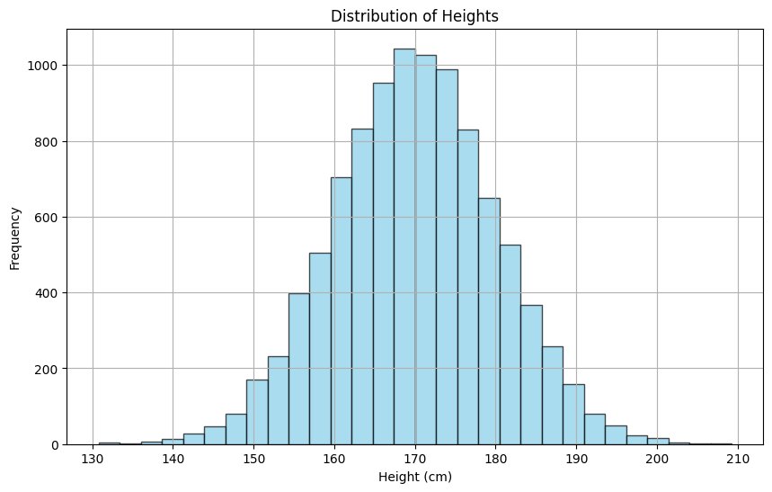Such a distribution looks like that a Gaussian measure of the form \[ p_{\mu, \sigma}(x) = \frac{1}{\sigma \sqrt{2\pi}} \exp\left(\frac{-(x-\mu)^2}{2\sigma^2}\right) \] where \(\mu\) is the average value and \(\sigma>0\) is the standard deviation around that average value. We can then try to find the best Gaussian approximation of our height distribution, that to find the best parameters \(\mu, \sigma\) so that \(p_{\mu, \sigma}\) would be more likely to produces our data \((x_i)_{i=1}^N\) as independent samples. Intuitively, one would choose \(\mu\) to be the empirical average of the data and \(\sigma^2\) to be the empirical variance around this empirical average value: \begin{align*} \overline{x} &= \frac{1}{N} \sum_{i=1}^{N}x_i \\ \overline{\sigma^2} &= \frac{1}{N} \sum_{i=1}^{N} (x_i - \overline{x})^2. \end{align*}

Remark

The reader familiar with statistics may use also the following variance estimator \[ \widetilde{\sigma^2} = \frac{1}{N-1} \sum_{i=1}^{N} (x_i - \overline{x})^2 \] which is unbiased, but is not what is provided by the maximum likelihood method.

A mathematical formulation : the maximum likelihood method.

Let us formulate this in mathematical terms. We have \(N\) samples in \(X\) that actually forms a single point \((x_i)_{i=1}^N\) in the product space \(X^N\). Our statistical model consists in a parametrized set of probabilities on \(X^N\) \[ p_\theta^{(N)}(z_1, \ldots, z_N), \ \theta \in \Theta, \ (z_1, \ldots, z_N) \in X^N \] where \(\Theta\) is the parameter space ; our goal is to find a parameter \(\widehat{\theta} \in \Theta\) that maximises the probability of the samples sequence \((x_i)_{i=1}^N\) \[ \widehat{\theta} = \mathrm{argmax}_\theta \left(p_\theta^{(N)}(x_1, \ldots, x_N) \right). \] In most case we assume that the samples are independent and identically distributed on \(X\). Putting that information into our statistical model just means that \(p_\theta^{(N)}(z_1, \ldots, z_N)\) has the form \[ p_\theta^{(N)}(z_1, \ldots, z_N) = \prod_{i=1}^N p_\theta(z_i) \] where \(p_\theta\) is a parametrized probability distribution on \(X\). In that context, we want to find \(\widehat{\theta}\) that maximises the model probability to get the actual samples \[ \mathcal L_\theta = \prod_{i=1}^{N} p_\theta(x_i) \] which is called the likelihood \(\mathcal L_\theta\). Equivalently, we want to maximize the log-likelihood which is the sum \[ \log\mathcal L_\theta = \sum_{i=1}^{N} \log(p_\theta(x_i)). \] Let us go back to the two examples of the first paragraph.

In the good/bad weather example, our statistical model is \[ p_\theta(\mathrm{good}) = \theta, \ p_\theta(\mathrm{good}) = 1- \theta, \ \theta \in [0, 1]. \] If we denote \begin{align*} g &= \#\{i|\ x_i = \mathrm{good}\} \\ b &= \#\{i|\ x_i = \mathrm{bad}\} = N-g, \end{align*} then the likelihood is \[ \mathcal{L}_\theta = \theta^g(1-\theta)^n \] and the unique parameter \(\widehat{\theta}\) that maximises this likelihood is the ratio \(\frac{g}{N}\) of days whose weather is good.
In the height distribution example, our statistical model is the set of Gaussian distributions \(p_{\mu,\sigma}\) parametrized by the mean value \(\mu\) and the standard deviation \(\sigma>0\) (or equivalently the variance \(\sigma^2\)). The log likellihood is the function \[ \log \mathcal{L}_{\mu, \sigma^2} = - \frac{N}{2}\log(2\pi) - N \log(\sigma) - \sum_{i=1}^{N} \frac{(x_i-\mu)^2}{2 \sigma^2} \] The parameters \((\mu, \sigma^2)\) that maximize the likelihood are those described in the first paragraph.

An information theoretical perspective.

We can imagine that our samples are produced independently by a probability distribution \(p\). In that context, a mathematical result called the large number theorem tells us that when \(N\) is large enough the normalized log-likelihood \(\frac{1}{N}\log \mathcal{L}_\theta\) converges to the expectation value of the quantity \(\log\left({p_\theta(x)}\right)\) for \(x\) distributed according to the probability distribution \(p\): \[ \frac{1}{N}\log \mathcal{L}_\theta = \frac{1}{N}\sum_{i} \log\left({p_\theta(x_i)}\right) \xrightarrow{N \to \infty} \int_{x \in X} p(x)\log\left({p_\theta(x)}\right) dx. \] The opposite of such a quantity is called the relative entropy of \(p\) with respect to \(p_\theta\): for two probability distributions \(q_1, q_2\) the relative entropy of \(q_1\) with respect to \(q_2\) is \[ H(q_1, q_2) = -\int_{x \in X} q_1(x)\log\left({q_2(x)}\right) dx = \int_{x \in X} q_1(x)\log\left(\frac{1}{q_2(x)}\right) dx. \] We can consider the relative entropy as some kind of distance between \(q_1\) and \(q_2\). However, it does have the usual properties of distances in mathematics. For instance, it is not zero when \(q_1=q_2\) but it is equal to the entropy of \(q_1\) \[ H(q_1) = H(q_1,q_1) = \int_{x \in X} q_1(x)\log\left(\frac{1}{q_1(x)}\right) dx. \] To fix that, we can substract the entropy \(H(q_1)\) from the relative entropy \(H(q_1, q_2)\) to obtain the Kullback Leibler divergence \[ KL(q_1||q_2) = H(q_1, q_2)-H(q_1) = \int_{x \in X} q_1(x)\log\left(\frac{q_1(x)}{q_2(x)}\right) dx. \] Nor is it a distance in the mathematical sense of the word but the concavity of the log function implies that

\(KL(q_1||q_2) \geq 0\);
\(q_1\) and \(q_2\) are almost surely equal if and only if \(KL(q_1||q_2) =0\).

One can thus see the goal of statistics as the minimisation with respect to \(\theta\) of the Kullback Leibler divergence \(KL(p||p_\theta)\) from the empirical probability distribution \(p\) to the model \(p_\theta\). In this line of thought, we do not have a direct access to \(p\) but only to its samples \((x_i)_{i=1}^N\) and by the law of large numbers \[ KL(p||p_\theta) = H(p, p_\theta) - H(p) \simeq \frac{1}{N}\log \mathcal{L}_\theta - H(p). \] Then we minize \(\frac{1}{N}\log \mathcal{L}_\theta - H(p)\) instead of \(KL(p||p_\theta)\) and hope that the two quantity are close enough so that this leads us to approximately minimise the Kullback Leibler divergence. Since \(H(p)\) is constant with respect to \(\theta\), we actually minimise \(\frac{1}{N}\log \mathcal{L}_\theta\) which is equivalent to minimising the log-likelihood \(\log \mathcal{L}_\theta\) or the likelihood \(\mathcal{L}_\theta\).

The Bayesian perspective and regularisation of parameters.

Let us shift our point of view towards the Bayesian perspective. In that perspective, before any knowledge on the samples, we postulate a probability distribution on \(X^N\) \[ q(z_1, \ldots, z_N),\ (z_1, \ldots, z_N) \in X^N \] that does not represent a fictional probability distribution that would produce the samples but rather our own expectation to see a particular set of samples appear; we use the letter \(q\) instead of the letter \(p\) to emphasize this shift in interpretation. In the context of parametrized Bayesian statistics and if we postulate independence of sample, \(q(z_1, \ldots, z_N)\) is built from a parametrized distribution \[ q_\theta(z_1,\ldots, z_N) = \prod_{i=1}^{N}q_\theta(z_i) \] that is, a set of distributions on \(X\) that depends on a parameter \(\theta \in \Theta\). Before seeing the actual samples, we have initially a vague idea of what the parameter \(\theta\) should be; and this idea is encoded in a probability distribution \(q_{\mathrm{prior}}(\theta)\) on \(\Theta\) called the prior probability. Combining the parametrized distribution \(q_\theta\) on \(X^N\) and the prior distribution \(q_{prior}(\theta)\) on \(\Theta\) gives us a probability distribution on the product \(X^N \times \Theta\) \[ Q(z_1, \ldots, z_N, \theta) = q_{\mathrm{prior}}(\theta) \prod_{i=1}^{N}q_\theta(z_i). \] Then, \(q(z_1,\ldots, z_N)\) is the marginal probability distribution on \(X^N\) from \(Q\): \begin{align*} q(z_1, \ldots, z_N) =& \int_{\theta \in \Theta} Q(z_1, \ldots, z_N, \theta)d\theta. \\ =&\int_{\theta \in \Theta} q_{\mathrm{prior}}(\theta) \times \prod_{i=1}^{N} q_{\theta}(z_i)d\theta. \end{align*} Moreover, \(q_\theta(z_1, \ldots, z_N)\) is actually the conditional probability distribution on \(X^N\) from \(Q\) with respect to \(\theta\) \[ q_\theta(z_1, \ldots, z_N) = Q(z_1, \ldots, z_N |\theta) = \frac{Q(z_1, \ldots, z_N, \theta)}{q_{\mathrm{prior}}(\theta)}. \] The effect of seeing the samples \((x_i)_{i=1}^N\) is to make us revise our view on on the parameters. Concretely, our new expectation on the parameters \(\theta \in \Theta\), that we call the posterior probability distribution \(q_{\mathrm{post}}(\theta)\), is the conditional probability from \(Q\) with respect to these samples \[ q_{\mathrm{post}}(\theta) = Q(\theta|x_1, \ldots, x_N) = \frac{Q(x_1, \ldots, x_N, \theta)}{q(x_1, \ldots, x_N)}. \] This can be rewritten (with the reknowned Bayes rule) as \[ q_{\mathrm{post}}(\theta) = \frac{q_{\mathrm{prior}}(\theta)\prod_{i=1}^N q_\theta(x_i)}{q(x_1, \ldots x_N)} = \frac{q_{\mathrm{prior}}(\theta)\mathcal{L}_\theta}{q(x_1, \ldots x_N)} \] where \(\mathcal{L}_\theta = \prod_{i=1}^N q_\theta(x_i)\) is the likelihood. The posterior probability is actually intractable in most real life contexts (as it requires to compute \(q(x_1, \ldots x_N)\) which is an integral). To circumvent this difficulty, we can instead search for the parameter value \(\widehat{\theta}\) that maximises the posterior probability distribution \(q_{\mathrm{post}}\) on the actual sample \(x_1, \ldots, x_N\); equivalently it maximises the product of \(q_{\mathrm{prior}}(\theta)\) with the likelihood \(\mathcal{L}_\theta\) (since \(q(x_1, \ldots x_N)\) does not depend on \(\theta\)); or taking the log, \(\widehat{\theta}\) maximises the sum \[ \log \mathcal{L}_\theta + \log(q_{\mathrm{prior}}(\theta)) = \sum_{i=1}^N \log(q_\theta(x_i)) + \log(q_{\mathrm{prior}}(\theta)). \] Such a method is called the maximisation a posteriori. The additional term \(\log(q_{\mathrm{prior}}(\theta))\) that reflects our prior beliefs on \(\theta\) is called the regularisation term. Usually, the more specific the prior is, the more this term pulls the maximum a posteriori parameter from the maximum likelihood parameter. In extreme cases:

when the prior distribution is a dirac measure at a value \(\theta_0\) (this means that we are absolutely certain that \(\theta_0\) is the relevant value), the maximum a posteriori parameter remains \(\theta_0\);
when the prior distribution is a uniform distribution reflecting our absence of prior knowledge, the maximum a posteriori parameter is equal to maximum likelihood value.

Let us apply this Bayesian perspective to our two examples.

In the first example dealing with good or bad weather, the parameter \(\theta\in [0,1]\) represents the probability of the weather to be good. With no prior knowledge about the weather, we can postulate a uniform prior probability on the set of parameters \[ q_{\mathrm{prior}}(\theta) = 1. \] In that context, if we actually observe \(g\) good weather days and \(b = N-g\) bad weather days, we get \[ q(x_1, \ldots x_N) = \int_{\theta \in [0,1]} \theta^g (1-\theta)^b d\theta = \frac{1}{g} - \frac{1}{N} = \frac{b}{Ng}. \] Then, the posterior probability distribution on the space of parameters \(\theta \in \Theta = [0,1]\) is \begin{align*} q_{\mathrm{post}}(\theta) &= \frac{q_{\mathrm{prior}}(\theta)\prod_{i=1}^N q_\theta(x_i)}{q(x_1, \ldots x_N)} \\ &= \frac{Ng}{b} \theta^g(1-\theta)^b \end{align*} Finally the maximum a posteriori parameter is \[ \widehat{\theta}_{\mathrm{MAP}} = \frac{g}{N}. \] It is equal to the maximum likelihood parameter since our prior probability distribution is the uniform one.
In the second example (the Gaussian fit), let us assume to make things simpler, that in our statistical model, the variance \(\sigma^2\) is no more a parameter but is fixed to \(1\). Subsequently this statistical model takes the form \[ q_\mu(z) = \frac{1}{\sqrt{2\pi}} \exp\left(-\frac{(z-\mu)^2}{2}\right); \] the unique parameter \(\mu\) is the average value of the parametrized distribution \(q_\mu\). Roughly, we can imagine that the average height is around \(\mu_0 = 1.5m\) with some uncertainty scale \(\alpha>0\); thus let us postulate a Gaussian prior distribution on \(\mu\) \[ q_{\mathrm{prior}} (\mu) = \frac{1}{\alpha\sqrt{2\pi}} \exp \left(-\frac{(\mu-\mu_0)^2}{2\alpha^2}\right) \] In that context, the likelihood and the regularisation term are \begin{align*} \mathcal{L}_{\mu} &= -\sum_{i=1}^{N} \frac{(x_i-\mu)^2}{2\sigma^2} + \mathrm{cst} \\ \log(q_{\mathrm{prior}}(\mu)) &= - \frac{(\mu-\mu_0)^2}{2\alpha^2} + \mathrm{cst} \end{align*} where the symbol \(\mathrm{cst}\) refers to some values that do not depend on \(\mu\). Thus, the maximum a posteriori parameter is \[ \widehat{\mu}_{\mathrm{MAP}} = \frac{N\alpha^2 \overline{x} + \mu_0}{N\alpha^2 + 1}. \] The factor \(N\alpha^2\) combines the number of samples with our initial uncertainty \(\alpha\). When it is high, meaning that the number of samples \(N\) is large enough to bend the strength \(1/\alpha^2\) of our initial beliefs, then \(\widehat{\mu}_{\mathrm{MAP}}\) converges to the maximum likelihood parameter \(\overline{x}\). When it is low, \(\widehat{\mu}_{\mathrm{MAP}}\) remains close to our first assumption \(\mu_0\).